Pest in R using R6 classes

Agent-based simulation of epidemics in R using OOP and R6 classes.

Author

Marcin Kierczak

Published

June 20, 2024

Modified

June 20, 2024

Hello! In this post, I will show you how one can implement an agent-based simulation in R using object-oriented programming paradigm (OOP) and R R6 classes. (

This simulation is working yet it still has to be polished. It has been implemented as a live coding demo during “OOP in R” session at RaukR 2024.

Our goal is to simulate epidemics dynamics on an island (an isolated world). Let us establish some simple rules:

we have a N x N squartes large rectangular world (think of each square as of, e.g. a building)
in each square dwell individuals that can be: healthy, immune (after recovering or vaccination), infected (= sick) or, unfortunately, also dead
in total, we have P individuals randomly distributed in our world’s squares
at every time step/round of our simulation individuals move and update their state
probability of becoming infected is proportional to the number of already infected individuals in the same square
probabilities of the remaining state transitions are given by simulation parameters
we continue the simulation for T rounds

An individual

Let’s begin by formulating an R6 class that represents an individual (= agent):

library(R6)

Agent <- R6Class("Agent",
  public = list(
    state = character(),
    initialize = function(state = "healthy") {
      self$state <- state
    },
    update_state = function(sick_prob, recovery_prob, death_prob) {
      # If agent is healthy it can either stay healthy or get infected
      if (self$state == "healthy") {
        new_state <- sample(x = c("healthy", "sick"), 
                       size = 1, 
                       prob = c(1-sick_prob, sick_prob))
      # A sick agent can continue being sick, recover and become immune or die
      } else if (self$state == "sick") { 
        new_state <- sample(x = c("sick", "immune", "dead"), 
                       size = 1, 
                       prob = c((1-(recovery_prob + death_prob)), recovery_prob, death_prob))
      
      } else {
        new_state <- self$state # Immune and dead states do not change
      }
      self$state <- new_state  # Update state
    }
  )
)

Observe that:

The default state of a new agent is “healthy”
We use sample and its prob argument to sample agent’s fate according to provided probabilities
“immune” and “dead” states do not change
when an individual is sick it can either continue to be sick, recover and become immune or die
we are using the fact that probabilities of mutually exclusive elementary events sum to 1

Simulation world

medieval-style cartoon map of the world Now it is time to create a class for our world which we can next populate with our agents. We need the following:

variable size where we store information about our world size N,
variable world which will store our representation of the world. Since the world is a square, we can use R base data structure – matrix and each cell in the matrix will contain a list of our individuals that dwell there – they are of class Agent that we have just created
method initialize that creates the world
method add_agent to populate our world
method move_agent to move agents around at each simulation step
method update_states that updates states of agents
method get_counts that will record current state of the world (count of healthy, sick etc.)

World <- R6Class("World",
  public = list(
    size = NULL,
    world = NULL,
    
    initialize = function(size) {
      self$size <- size
      self$world <- matrix(vector("list", size * size), nrow = size, ncol = size)
      for (i in 1:size) {
        for (j in 1:size) {
          self$world[[i, j]] <- list()
        }
      }
    },
    
    add_agent = function(row, col, agent) {
      self$world[[row, col]] <- c(self$world[[row, col]], list(agent))
    },
    
    move_agents = function() {
      new_world <- matrix(vector("list", self$size * self$size), nrow = self$size, ncol = self$size)
      for (i in 1:self$size) {
        for (j in 1:self$size) {
          agents <- self$world[[i, j]]
          for (agent in agents) {
            if (agent$state != "dead") { # dead do not move
              move <- rnorm(2, mean = 0, sd = 1) # some arbitrary motility
              new_row <- min(max(1, round(i + move[1])), self$size)
              new_col <- min(max(1, round(j + move[2])), self$size)
              new_world[[new_row, new_col]] <- c(new_world[[new_row, new_col]], list(agent))
            } else {
              new_world[[i, j]] <- c(new_world[[i, j]], list(agent))
            }
          }
        }
      }
      self$world <- new_world
    },
    
    update_states = function(beta, recovery_prob, death_prob) {
      # Iterate over all grid cells in the world and 
      # determine infection probability based on
      # the number of already sick individuals in that grid cell.
      for (i in 1:self$size) {
        for (j in 1:self$size) {
          agents <- self$world[[i, j]]
          num_sick <- sum(vapply(agents, function(agent) agent$state == "sick", logical(1)))
          # Now, probability of becoming sick is naively proportional 
          # to the percentage of already sick individuals in the cell
          # where beta is the transmission probability
          sick_prob <- 1 - ((1 - beta) ^ num_sick)
          for (agent in agents) {
            agent$update_state(sick_prob, recovery_prob, death_prob)
          }
        }
      }
    },
    
    get_counts = function() {
      counts <- data.frame(
        row = integer(),
        col = integer(),
        healthy = integer(),
        immune = integer(),
        sick = integer(),
        dead = integer()
      )
      for (i in 1:self$size) {
        for (j in 1:self$size) {
          agents <- self$world[[i, j]]
          counts <- rbind(counts, data.frame(
            row = i,
            col = j,
            healthy = sum(vapply(agents, function(agent) agent$state == "healthy", logical(1))),
            immune = sum(vapply(agents, function(agent) agent$state == "immune", logical(1))),
            sick = sum(vapply(agents, function(agent) agent$state == "sick", logical(1))),
            dead = sum(vapply(agents, function(agent) agent$state == "dead", logical(1)))
          ))
        }
      }
      return(counts)
    }
  )
)

Tip

One line of code is probably a bit non-intuitive:

sick_prob <- 1 - ((1 - beta) ^ num_sick)

Here, parameter beta (\(\beta\)) is the so-called transmission probability that is specific for each disease agent. Now, \(P({not\_sick}) = (1 - \beta)^{N_{sick}}\) is the probability of NOT catching the disease from any of \(N_{sick}\) neighbors. Finally, the chance of becoming sick in a given cell is \(P_{sick} = 1 - P({not\_sick}) = 1 - (1 - \beta)^{N_{sick}}\)

Auxiliary functions

I have written a function that visualizes states of our world as the simulation goes on using ggplot2 and gganimate packages. Here is the code:

visualize_simulation <- function(results) {
  p <- ggplot(results, aes(x = col, y = row)) +
    geom_tile(aes(fill = sick)) +
    scale_fill_gradient(low = "white", high = "red") +
    theme_minimal() +
    labs(title = "Disease Spread Simulation", x = "X", y = "Y", fill = "Sick Individuals") +
    transition_states(step, transition_length = 2, state_length = 1) +
    ease_aes('linear') +
    ggtitle('Disease Spread Simulation - Generation {closest_state}') +
    theme(plot.title = element_text(size = 16, face = "bold", hjust = 0.5))
  
  animate(p, nframes = length(unique(results$step)), fps = 2, renderer = gifski_renderer())
}

Running simulation

Now, we need a function that will enable us to run the simulation:

library(ggplot2)
library(gganimate)
library(progress)

run_simulation <- function(size, num_steps, initial_immune, initial_sick, beta, recovery_prob, death_prob) {
  stopifnot(recovery_prob + death_prob <= 1) # some simplistic input validation
  pb <- progress_bar$new(total = num_steps + 1)
  
  world <- World$new(size)
  
  # Initialize agents
  if (initial_healthy > 0) {
    for (i in 1:initial_healthy) {
      row <- sample(1:size, 1)
      col <- sample(1:size, 1)
      world$add_agent(row, col, Agent$new())
    }
  }
  
  # Introduce immune and sick agents
  if (initial_immune > 0) {
    for (i in 1:initial_immune) {
      row <- sample(1:size, 1)
      col <- sample(1:size, 1)
      world$add_agent(row, col, Agent$new(state = "immune"))
    }
  }
  
  if (initial_sick > 0) {
    for (i in 1:initial_sick) {
      row <- sample(1:size, 1)
      col <- sample(1:size, 1)
      world$add_agent(row, col, Agent$new(state = "sick"))
    }
  }
  
  results <- list()
  
  # Save the initial state of the world
  counts <- world$get_counts()
  counts$step <- 1
  results[[1]] <- counts
  
  
  # Simulate one generation
  for (step in 2:num_steps + 1) {
    world$update_states(beta, recovery_prob, death_prob)
    world$move_agents()
    counts <- world$get_counts()
    counts$step <- step
    results[[step]] <- counts
    pb$tick()
  }
  
  results <- do.call(rbind, results)
  
  return(results)
}

Finally, we can run our simulation:

library(tidyverse)

── Attaching core tidyverse packages ──────────────────────── tidyverse 2.0.0 ──
✔ dplyr     1.1.4     ✔ readr     2.1.5
✔ forcats   1.0.0     ✔ stringr   1.5.1
✔ lubridate 1.9.3     ✔ tibble    3.2.1
✔ purrr     1.0.2     ✔ tidyr     1.3.1
── Conflicts ────────────────────────────────────────── tidyverse_conflicts() ──
✖ dplyr::filter() masks stats::filter()
✖ dplyr::lag()    masks stats::lag()
ℹ Use the conflicted package (<http://conflicted.r-lib.org/>) to force all conflicts to become errors

# Parameters
size <- 20                    # World size
num_steps <- 50               # Number of generations
initial_healthy <- 998
initial_immune <- 0
initial_sick <- 2
beta <- 0.5                  # Transmission probability
recovery_prob <- 0.1
death_prob <- 0.05

# Run the simulation
results <- run_simulation(size, num_steps, initial_immune, initial_sick, beta, recovery_prob, death_prob)

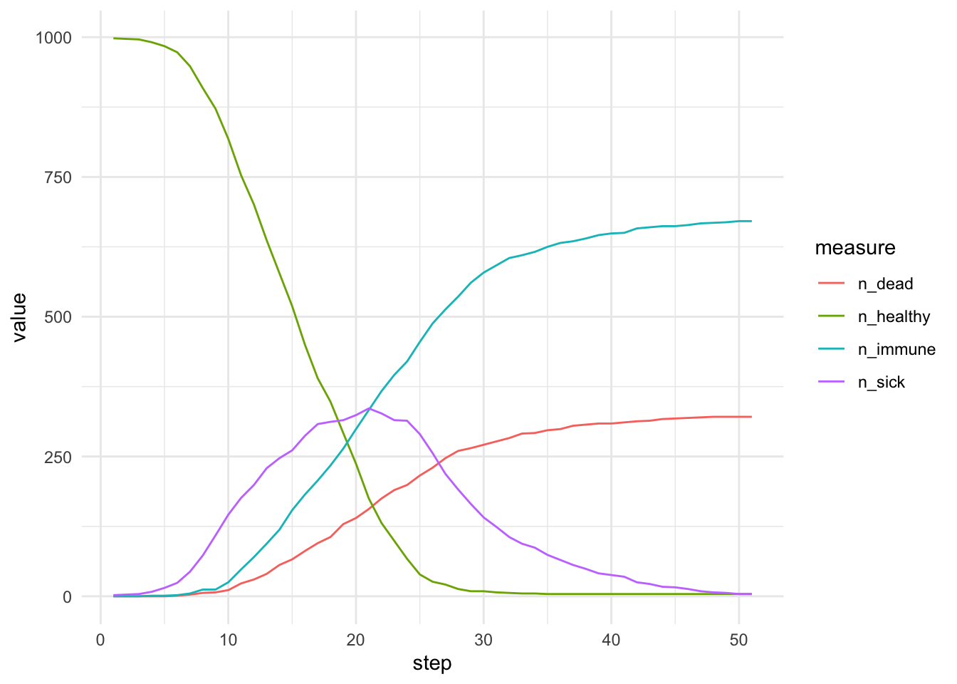
results |> group_by(step) |> 
  summarise(n_sick = sum(sick), n_healthy = sum(healthy), n_immune = sum(immune), n_dead = sum(dead)) |> 
  pivot_longer(starts_with("n_"), names_to = 'measure') |> 
  ggplot(aes(x = step, y = value, col=measure)) + geom_line() + theme_minimal()